If...if...We didn't love freedom enough. And even more, we had no awareness of the real situation.... We purely and simply deserved everything that happened afterward.
If...if...We didn't love freedom enough. And even more, we had no awareness of the real situation.... We purely and simply deserved everything that happened afterward.
Table of Contents
Introduction
What’s a skyrmion, anyway?
Topological Trivia
What’s a magnetic skyrmion?
Monte-Carlo Simulations and the Metropolis algorithm
GPU-based parallelization


From Autumn 2020 to Spring 2021, I wrote some software to simulate
physical structures called magnetic skyrmions. The software used a
Monte-Carlo method called the Metropolis-Hastings algorithm, which
‘probabilistically iterates the state of a simulated physical system in
such a way as to (hopefully) reach its ground state (the point with the
lowest energy)’.
(In other words, it’s a hill-climbing algorithm for very
high-dimensional configuration spaces.)
This had been done before, and was nothing special- skyrmion simulations were being run all the time. What made my code special was that I came up with a particular parallel version of the Metropolis-Hastings algorithm, inspired by the work of some Italians looking at the Ising model, and implemented this parallel algorithm on the GPU. This led to large speedups.
The point of this page is to explain the concepts mentioned above, describe the code I wrote, and reflect what I’ve learned from the experience.
(For more images like the ones you see above and throughout this
page, go here)
(I’ve also made a
short video showing a 2D skyrmion simulation in progress.)
A magnetic skyrmion is a skyrmion, but in a magnet!

First we need to talk about what a skyrmion is, and so we need to talk about this guy:

Tony Skyrme was a theoretical physicist born in 1922.
From 1958 to 1962, he published a series of six papers in which he tried
to rebuild particle physics from the ground up. 1
Briefly, Skyrme had some problems with contemporary particle theory 1 :
– Point particles. They’re infinitely dense, so they require
renormalization - dealing with the infinities you get in the
calculations relating to them, which Skyrme felt was hack-y
– Fermions and Bosons being separate fields. Skyrme wanted to see if he
could portray every particle as arising from the same
fundamental field.
– Fermions existing as ontologically separate particles at all! In his
own words:
“I have always felt an unease about quantum-mechanical concepts that do not have clear classical analogues”. 2
So Skyrme imagined a universe whose fundamental components weren’t point particles, but instead had a real size, a structure distributed across a finite amount of space. The particles he came up with were excitations in a fundamental field- like conventional point particles. The difference is that Skyrme’s distributed particles were stabilised by their topology- their shape. They were stable in the same way a knot in a loop of rope is..


Take the above image. A torus can’t deform into a sphere without breaking a surface- it can’t change into a sphere via ‘smooth’ deformations. Physical fields also change smoothly over time, without discontinuities, so no ‘tearing’ of the field’s fabric occurs. This means there are analogous configurations of the field
If you have two classes of field configuration that can’t be smoothly deformed into each other (this is referred to as two configurations having different homotopy groups), then a field configuration from class A is stable in the particular sense it’ll never turn into a field configuration from class B.
Topological Trivia (click to expand)
In topology, a map is a function that associates points in one space with points in another (or the same). Two maps are homotopic if one can be smoothly deformed into one another. for example, maps from to , and from to . The map can be smoothly deformed into the map ;
for Is a continuous function of t, and is equal to and for and respectively. Hence and are homotopic.
Certain collections of maps can be split into homotopy classes, defined such that all maps in the same class are mutually homotopic and maps in different classes are not.
One example of a map is a continuous map from one circle to another, say , where represents a point on the the first circle such that with
Where k is an integer, meaning the function is continuous over whole the domain circle: there is no ‘jump’ in the angular value at any point. This constraint is key.
We can now define a ‘winding number’, the number of times the range circle is traversed over one traversal of the domain circle:The earlier continuity constraint means that the winding number must be an integer.
One cannot smoothly deform a map with one winding number to one with another while obeying this continuity constraint: the value of would have to either jump (a discontinuity in the deformation) or have a smoothly varying value of (breaking the continuity of on the domain circle).
This property partitions the space of functions/maps into ‘homotopy classes’- sets of maps that can smoothly deform into one another. Imagine that represents the state of some field at a certain point in time, such that it could smoothly deform according to some equation of motion that includes embedded this continuity constraint.
The field could change, but the winding number would be a conserved value.
If a loop of rope has a winding number of zero, a loop with one
overhand knot has one, a rope with two has two… given the overall rope
is a loop, you can’t globally make or undo any topologically nontrivial
knots without breaking the rope. Use this as a crude, horrible analogy
for a field and we now have a conservation law: the net ‘topological
charge’ of the field (its winding number) is neither created nor
destroyed.
Skyrme then said that particles are (local) field configurations that
aren’t homotypes of the vaccum (flat) field configuration; different
particles are field configurations with different topological charges.
These particles would be stable because there’s no topological path from
them to the vacuum state. Another term for these particles is
‘topological solitons’.
Clearly, this isn’t how most people imagine fundamental particles
today, and Skyrme died of surgical complication in the 80s at only
64.
However, after his death, his ideas of distributed structures stabilised
by topology remained of interest, and the word ‘skyrmion’ was coined for
topologically stabilised particles or quasiparticles.
Then, people found skyrmions in ferromagnets.
In contrast to Skyrme’s fundamental particle candidates, which are patterns in bosonic fields, magnetic skyrmions are topologically stabilised ‘spin textures’ inside magnetic materials: patterns in the magnetic field inside a material, in particular a pattern in the directions of atomc spins.
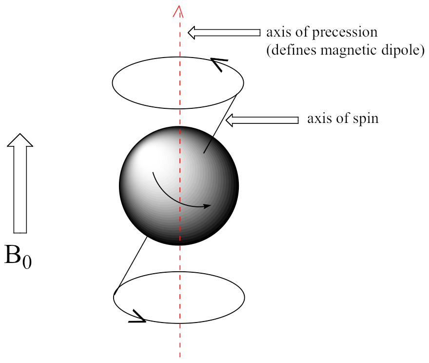
Atoms have magnetic dipoles, and you can classically model atoms in solids as tiny bar magnets rotating back and forth, magnetically pushing and pulling on each other. The axis of the atom’s magnetic dipole is also referred to as the axis of the atom’s ‘spin’, as that’s what the dipole is, quantum-mechanically (although the spin vector is opposite to the magnetic dipole vector).
In a crystalline magnetic solid, atoms are arranged in a lattice such that each atom’s spin-vector rotates in interaction with the surrounding magnetic environment, including other (primarily neighbouring) spins. Such an arrangement is known as a spin lattice.

Left: a representation of a
2-dimensional 7x7 spin lattice. Coloured spin vectors are examples of
pairs that are nearest-neighbours only under periodic boundary
conditions. Right: a representation of a 3-dimensional 4x4x4 spin
lattice.
If atoms are like little bar magnets (in this classical approximation,
disregarding most quantum effects), then we might imagine this
arrangement is like having lots of little bar magnets on gimbals in a
lattice. You’d expect the bar magnets to push and pull on each other,
with magnets close together ‘wanting’ to end up end-to-end.
Ferromagnetic materials have the property that neighbouring spins tend to align, giving rise to macroscale magnetism when enough spins are coaligned. Under specific conditions, in specific materials, more complicated spin configurations- spin textures- can arise.
In the late 1970s, small angle neutron scattering experiments found helical (rotating) spin textures in chiral ferromagnets such as MnSi . In order to explain these structures and predict others, Ginzburg-Landau theories were constructed for these materials. Over the course of the next decade, these theories expanded to include the Dzyaloshinskii-Moriya interaction, which could only appear in chiral magnets and was deemed critical for the formation of helical structures, and the influence of an external magnetic field. Based on these theories, it was predicted that magnetic skyrmions would be found within given ranges of external field strengths in certain materials.
The ‘A-phase’ of MnSi, a region within a small window of temperature and applied field strength, was predicted to host skyrmions, and eventually this was confirmed by neutron scattering experiments.
Magnetic skyrmions are quasiparticle spin textures observed in
certain magnetic materials; large-scale patterns (on the order of tens
of atoms) in the orientations of spins that can persist and migrate
through the spin lattice, forming, combining, and annihilating like
particles. Magnetic skyrmions are obviously not indestructable; the
underlying substrate is not ‘smooth’, consisting of a lattice of atoms,
and can be overridden by brute force (a very strong magnetic field).
However, they are topologically protected. Like their older
counterparts, magnetic skyrmions have an associated winding numbers;
nonzero integer winding numbers, to be precise. Different winding
numbers produce different skyrmion patterns.
The topological protection manifests itself as an energy barrier. This grants them high metastability: they can survive for a long time even when not being the ground state.
The presence of magnetic skyrmions within chiral ferromagnets such as MnSi is due to the latter’s micromagnetic properties that give rise to energetic interactions that stabilise the skyrmion phase. As such, skyrmions will form spontaneously within specific ranges of temperature (T) and applied external magnetic field (B), i.e. the A-phase, henceforth the skyrmion phase. Due to their metastability, they can then go on to survive for some time outside of the regions in which they form.
We use a simplified lattice model and discrete Hamiltonian to model
the interactions in skyrmion-bearing materials, allowing us to estimate
the ground state of the system for a given value of (T,B) using the
Metropolis-Hastings algorithm, a type of Monte Carlo method.
We use Graphical Processing Units (GPUs) to parallelize and thus speed
up these simulations.
You can see the link between electron spin and magnetic moments by looking at Maxwell’s law
We use a parallelized variant of a Monte Carlo method called the single spin-flip Metropolis algorithm to simulate our spin-system. The Metropolis-Hastings algorithm takes a starting state, a function that randomly perturbs this state, and a target distribution, and evolves the starting state such that eventually, successive iterations of the state are samples from the target distribution. One useful property of the algorithm is that the target distribution only has to be known up to a multiplicative constant.
In our case,
– The configuration space is the that of our model, which has
degrees of freedom
– The method for perturbing the state is by ‘flipping’ a given spin to a
random orientation
– The target distribution has high measure has greater measure for lower
energies, down to a minimum energy defined by a temperature constant
The Metropolis algorithm for iterating the state is:
– Pick a spin vector (a lattice point) at random
– Randomly generate a new unit vector
– If
Replace the old vector with the new one; else, do so with
probability
Where and are the energy of the system according to the HMDZ Hamiltonian:
We can note that for any given proposed spin-flip, the difference in
overall energy depends only on the terms that include the flipped spin.
Thus we don’t need to calculate the Hamiltonian for the entire spin
lattice in order to calculate the difference between the old and new
energies, but merely the terms including the proposed and old
spins.
From the point of view of computer memory, this means we don’t have to
read to or write from any spins not interacting with the current spin
under consideration in order to run an iteration of the Metropolis
algorithm.
This will be critical in our application of parallelism.
I implemented the parallel simulation algorithm using OpenGL compute shaders. I used these as opposed to CUDA (or OpenCL) for several reasons
1.) OpenGL works everywhere as opposed to only on Nvidia GPUs
2.) Rendering- the code runs quickly enough you can render the skyrmion simulation in real-time and interact with it live.
The local version of the code draws the simulation state and allows the user to manipulate simulation parameters in real-time, moving the camera around, etc. I found this very helpful for gaining practical understanding; being able to watch the skyrmion state nucleate (form) and collapse in realtime was informative. Additionally, there’s a keybind to save the simulation state at will, so I could observe a simulation run (~2 minutes) and manually save the most interesting configurations for later analysis. This would have been possible using CUDA for the simulation, but I’d still have had to use openGL or similar to render, so I found it easier to do it all with one library.
3.) I’m more familiar with openGL than CUDA, and given I was writing nontrivial code in C, I needed all the development speedup I could get!
Earlier, I talked about how stable skyrmions are. The good news is,
this was reflected in my simulations! The bad news is, this was
reflected in my simulations. Remember, the goal was to find the
minimum-energy state for each point in B-T space, and we do this using a
probabilistic hill-climbing (descending) algorithm called the Metropolis
algorithm that follows energy gradients down and can sometimes jump up
small gradients. The reason skyrmions are stable is because there’s a
large energy barrier between them and any lower-energy states.
This means that small perturbations to the skyrmion state just collapse
back into it. Unfortunately for us, this applies to the Metropolis
algorithm, too.
For the same reasons that skyrmions are interesting in real life, they’re also troublesome to our simulation! When the simulation state gets went into the skyrmion phase (by moving into the skyrmion-generating pocket of B-T space), I found it almost impossible to get rid of them by moving out again- except by ramping the temperature high enough to re-randomize the whole system. This is, of course very annoying, because it means you get phase diagrams like this:


Here, we reach every point by setting B to a fixed value and slowly decreasing T. You can see that every path that passes through the skyrmion phase ‘catches’ skyrmions and keeps them. As you can see, this somewhat matches the black and white phase diagram from pre-existing Monte-Carlo simulation work done by Buhrandt and Fritz, but not entirely.
1 Skyrme, T H.R., The origins of Skyrmions,
doi: 10.1142/S0217751X88001156, International Journal of Modern Physics
A, 1988
2 <sub id=“ref-3> 3 Buhrandt & Fritz, Skyrmion lattice phase in
three-dimensional chiral magnets from Monte Carlo simulations,
doi:10.1103/physrevb.88.195137, 2013